Rental Bike Demand Prediction
For a bike renting system to smoothly function, it is necessary to provide a stable supply of rental bikes at any given point of time according to the demand. This requires having a good prediction of the bike demand at each hour. I am working with a dataset of bike rental counts in the city of Seoul, South Korea which contains historical data on date and weather information (Temperature, Humidity, Windspeed, Visibility, Dewpoint, Solar radiation, Snowfall, Rainfall).
Overview
- The distributions of the features as well as their relationship with the rented bike count is explored.
- Linear regression model is trained on the data to make predictions and its performance is evaluated.
- Decision Tree Regression model is trained for getting better predictions and this model’s performance is evaluated as well.
- Python libraries such as Matplotlib, Seaborn, Pandas and Scikit-learn are used.
View the complete notebook HERE
Data Source
The dataset was obtained from UCI Machine Learning Repository GO TO SOURCE.
Relevant papers mentioned in the UCI Machine Learning Repository page [1] [2].
Objective
The aim is to predict the demand of rental bikes at any given hour using the weather and date information provided in the dataset.
Data Preparation
- The dataset column names were simplified.
- Date string values were converted to datetime format in order to retireve month and year information.
- There were no missing values to deal with in the dataset.
Exploratory Data Analysis
- Distribution of data across categories of various features was studied.
- Distribution of total rented bike counts across categories of features was explored.
- Relationships between the dependent variable and numerical features were visualised.
- Distributions of numerical features were visualised.
- Correlation between dependent and independent variables were calculated.

Model Fitting
Linear Regression Model
- Label encoding and one hot encoding was done on categorical variables.
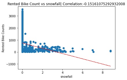
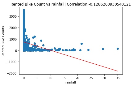
- Rainfall and snowfall variables were ignored as their relationship with the dependent variable is not linear.
- The dataset was split into training and testing dataset and scaled.
- The model was fit and the target variable predictions were made.
- Model performance was evaluated.
from sklearn.model_selection import train_test_split
from sklearn.preprocessing import MinMaxScaler
from sklearn.linear_model import LinearRegression
from sklearn.metrics import r2_score, mean_squared_error

# splitting data into training and testing set
X_train, X_test, y_train, y_test = train_test_split(X,y, test_size = 0.2, random_state = 4)

# scaling the data
scaler = MinMaxScaler()
X_train = scaler.fit_transform(X_train)
X_test = scaler.transform(X_test)

# fitting the model
linear_regressor = LinearRegression()
linear_regressor.fit(X_train, y_train)

# prediction using the model
y_pred = linear_regressor.predict(X_test)
y_train_pred = linear_regressor.predict(X_train)

# Performance metrics for testing data
# root mean squared error
print('RMSE:', math.sqrt(mean_squared_error(y_test, y_pred)))
# r2 score
print('R2 score:', r2_score(y_test, y_pred))

# Performance metrics for training data
# root mean squared error
print('RMSE:', math.sqrt(mean_squared_error(y_train, y_train_pred)))
# r2 score
print('R2 score:', r2_score(y_train, y_train_pred))
Performance metrics for Testing dataset
RMSE: 454.3735647954152
R2 score: 0.5117558744340127
Performance metrics for Training dataset
RMSE: 436.9096921808084
R2 score: 0.534370487444807
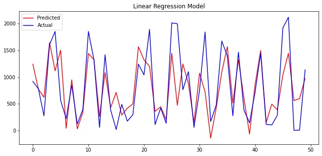
Comparison between actual and predicted values
Comparing the values visually using a snippet (first 50 values) of the actual and predicted values.
Decision Tree Regression Model
- Label encoding was done as Scikit-learn decision tree regressor does not support categorical variables.
- GridSearchCV was used for hyperparameter tuning and cross validation.
- The model was fit and the target variable predictions were made.
- Model performance was evaluated.
- The best hyperparameter combination (as given by GridSearchCV) was used to train a Decision Tree model in order to visualise the Tree.
from sklearn.tree import DecisionTreeRegressor
from sklearn.model_selection import GridSearchCV

# GridSearchCV for hyperparameter tuning
decision_tree_reg = DecisionTreeRegressor()
grid_parameters = {"max_depth": [3, 5, 7], "max_leaf_nodes": [None, 50, 60, 70, 80, 90], "min_samples_leaf":[7,8,9,10]}
regressor_model = GridSearchCV(decision_tree_reg, param_grid = grid_parameters, scoring = 'neg_mean_squared_error', cv = 5)

# fitting the model
regressor_model.fit(X_train2, y_train2)
Performance metrics for Testing dataset
r2 score: 0.7805191405790043
RMSE: 304.0104231418782
Performance metrics for Training dataset
r2 score: 0.8328601459379475
RMSE: 261.2260801680112
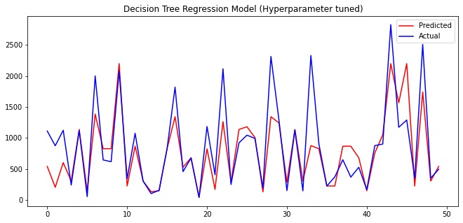
Comparison between actual and predicted values
Comparing the values visually using a snippet (first 50 values) of the actual and predicted values.
# best hyperparameters
regressor_model.best_params_
‘max_depth’: 7, ‘max_leaf_nodes’: None, ‘min_samples_leaf’: 8
Decision Tree Visualisation
A single decision tree model is trained using the best hyperparameter combination.
# fitting the model
decision_tree_model = DecisionTreeRegressor(max_depth = 7, max_leaf_nodes = None, min_samples_leaf = 8)
decision_tree_model.fit(X_train2, y_train2)

# visualising decision tree
from sklearn.tree import export_graphviz
import graphviz
from IPython.display import Image

dot_data = export_graphviz(decision_tree_model, feature_names=X_train2.columns, filled=True, out_file=None)
graph = graphviz.Source(dot_data)
png_img = graph.pipe(format='png')
Image(png_img)
Decision Tree
Click HERE to enlarge Image:

Conclusions
Exploratory Data Analysis
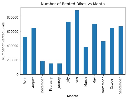
- June followed by July and May (summer season) has the most bikes rented. January, February and December (winter) has the least number of bikes rented.
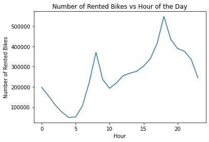
- The peak time of the day rented bike count is around 4-7 pm in the evening. There is a smaller peak in the morning (around 7-9 am). The least activity is during the early morning period.
- Summer is the most active season and winter is the least active one.
- Very low number of bikes were rented during holidays.
- There was a weak linear relationship with some of the variables. However, there was high standard deviation and high heteroskedasticity.
- Rainfall and snowfall variables had a non linear relationship with rented bike counts.
- The distribution of the dependent variable was skewed.
Linear Regression
- The model had an R2 score (Coefficient of determination) of 0.51 on testing set and 0.53 on training set i.e the model is able to explain around 51% of the variation in the predicted variable.
- The root mean squared error was found to be 454.37 on testing set and 436.90 on training set.
- The performance of the model on testing and training datset is fairly similar.
Decision Tree Regression
- The hyperparameter tuned model gave an R2 score of 0.779 on testing set and 0.832 on training set.
- The root mean squared error was 304.42 on testing set and 261.22 on training set.
- The best parameters were ‘max_depth’: 7, ‘max_leaf_nodes’: None, ‘min_samples_leaf’: 8.
References
[1] Sathishkumar V E, Jangwoo Park, and Yongyun Cho (2020). ‘Using data mining techniques for bike sharing demand prediction in metropolitan city.’ Computer Communications, Vol.153, pp.353-366.
[2] Sathishkumar V E and Yongyun Cho (2020). ‘A rule-based model for Seoul Bike sharing demand prediction using weather data’ European Journal of Remote Sensing, pp. 1-18.